clusterpathRcpp code analysis
1. $\ell_1$ penalty clustering method
$\ell_1$正则项的聚类效果。这一问题的的目标函数可以写成, \[ \sum_{k=1}^p \left[ \frac{1}{2} \sum_{i=1}^n (\alpha_{ik}-X_{ik})^2 +\lambda \sum_{i<j} w_{ij} \lvert \alpha_{ik}-\alpha_{jk} \rvert \right] = \sum_{k=1}^p f_1(\alpha^k,X^k) \] 其中,$\alpha^k \in \mathbb{R}^n$是$\alpha$的第$k$列。 这样,关于矩阵$X$的最小化问题就等价于$p$个分隔开的最小化子问题, \[ \min_{\alpha \in \mathbb{R}^{n\times p}} f_1(\alpha,X)=\sum_{k=1}^p \min_{\alpha^k \in \mathbb{R}^n} f_1(\alpha^k,X^k) \] 对于每一个子问题,可以使用FLSA path algorithm来解决。详细的理论分析将会在文章的后面部分给出。现在先从实验上有一个大致的直觉印象。在R环境中,执行以下代码。
library(clusterpathRcpp)
x <- c(-3,-2,0,3,5)
df <- clusterpath.l1.id(x)
plot(df)
得到的聚类结果为:
> df
   alpha    lambda row     col gamma norm solver
1    0.6 1.1333333   1 alpha.1     0    1   path
2    0.6 1.1333333   2 alpha.1     0    1   path
3    0.6 1.1333333   3 alpha.1     0    1   path
4    0.6 1.1333333   4 alpha.1     0    1   path
5    0.6 1.1333333   5 alpha.1     0    1   path
6    0.0 0.8333333   1 alpha.1     0    1   path
7    0.0 0.8333333   2 alpha.1     0    1   path
8    0.0 0.8333333   3 alpha.1     0    1   path
9   -1.0 0.5000000   1 alpha.1     0    1   path
10  -1.0 0.5000000   2 alpha.1     0    1   path
11  -3.0 0.0000000   1 alpha.1     0    1   path
12  -2.0 0.0000000   2 alpha.1     0    1   path
13   0.0 0.0000000   3 alpha.1     0    1   path
14   1.0 1.0000000   4 alpha.1     0    1   path
15   1.0 1.0000000   5 alpha.1     0    1   path
16   3.0 0.0000000   4 alpha.1     0    1   path
17   5.0 0.0000000   5 alpha.1     0    1   path
以及plot出来的效果:
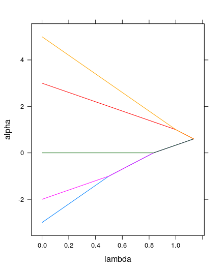
很明显,这是一个针对只有一维特征的数据矩阵(向量)的$\ell_1$的聚类算法执行结果。从结果到图形,光看最后那一句肯定是会蒙圈的,至少,我刚看到的时候是晕的。这里面包含了好几个代码上的trick。下面将一一解开。
1.1. R代码分析
把上述代码保存至一个R文件中,并使用调试模式(如果不会,可以自行度娘或勾勾,关键词“R, Rstudio, debug”)。先解决这个图是怎么画出来的吧!这个比较容易点,相对来说更直观的感受到R数据展示(绘图)的强大!导航至plot(df),跟进(step into function “SHIFT+F4”),得到如下代码,
function (x, type = "l", main = "The entire regularization path of optimal solutions for each variable",
	xlab = expression(paste("location in the regularization path  ",
		lambda)), ylab = expression(paste("optimal coefficient  ",
		alpha)), strip = strip.custom(strip.names = TRUE), layout = c(1,
		nlevels(x$col)), ...)
{
	xyplot(alpha ~ lambda | col, x, group = row, type = type,
		layout = layout, xlab = xlab, ylab = ylab, main = main,
		strip = strip, ...)
}
是不是和想像的不一样?原来clusterpathRcpp重新定义了plot。。。套路太深,有点想回农村,有木有!看到的不一定是你想的那样的,还是too young。。。有了df的结果数据,和plot的逻辑,可以自已去plot的玩了。比如”type=’p’”, 把col去掉,group=row去掉,还可以把xyplot换掉等等。不会玩的可以看R Graph 。
下面重点来了,这个算法是怎么处理数据的呢?导航至df<-clusterpath.l1.id(x),可以看到clusterpath.l1.id这个函数的具体内容:
function (x, LAPPLY = if (require(multicore)) mclapply else lapply)
{
  x <- as.matrix(x)
  dfs <- LAPPLY(1:ncol(x), function(k) {
    L <- .Call("join_clusters_convert", x[, k], PACKAGE = "clusterpathRcpp")
    data.frame(L[1:2], row = factor(L$i + 1), col = factor(k),
      gamma = factor(0), norm = factor(1), solver = factor("path"))
  })
  df <- do.call(rbind, dfs)
  if (!is.null(rownames(x)))
    levels(df$row) <- rownames(x)
  levels(df$col) <- alphacolnames(x)
  d <- structure(df, data = x, class = c("l1", "clusterpath",
    "data.frame"))
  unique(d)
}
可以看出,clusterpath.l1.id调用了lapply这个函数,而这个函数的主要作用是,对第一个参数1:ncol(x)的每一个成员执行function(k),这里k是形参,接收1:ncol(x)中的每一个具体值,处理完后返回一个和1:ncol(x)维度一致的结果向量。1:ncol(x)显然是一个数字序列,代表数据集x的每一列。而function(k)则是对每一列数据按特定的逻辑处理。这一逻辑正是C++函数join_clusters_convert。继续跟进join_clusters_convert,了解这个逻辑是怎么处理的?想法是好的,现实是残酷的。如果是matlab,这是可能的,但在R环境下,实在是没找到怎么调试的办法。或许我太嫩,调试方法羞于见我也说不定!有知道的GGJJDDMM可以联系我啊,万分感谢!直接调试,不太可能,辣么,可不可以在C++环境中调试呢?答案是”当然可以!“。可见,前期工作也没白费,正好派上用场。
下面就快速用codeblocks搭建好环境,当然是选择ubuntu啦!没有为什么,就特么用的爽!具体步骤可以参考Cpp invoke R library。 环境搭建好之后,来看一看我们的测试代码。
#include <iostream>
#include "interface.h"

#include <Rcpp.h>
#include <RInside.h>
#include <iomanip>

using namespace std;

int main(int argc, char* argv[])
{
    RInside R(argc,argv);
    std::string txt2 =
        "suppressMessages(library(clusterpathRcpp))";
    R.parseEvalQ(txt2);
    Rcpp::NumericVector dt((SEXP) R.parseEval("dt<-c(-3,-2,0,3,5)")); //iris[,1]"));
    R["res1"]=join_clusters_convert(dt);  //SEXP类型可以和R中的对象互转

    std::string txt3=
        "cat('\nres1=\n'); print(res1)";//[1:200,])";
    R.parseEvalQ(txt3);
    return 0;
}
是不是相当的easy? 程序猿都是活雷锋,RInside, Rcpp, 简直是太TM好用了!若对代码有疑问,请移步Cpp invoke R library。
1.2 C++代码分析
先来看一下涉及到的数据结构:
struct Cluster;
// Doubly-linked list of clusters
typedef std::list<Cluster*> Clusters;
// events are represented as a map, thus e->first is lambda and
// e->second is the pointer to the top cluster of the merge event.
typedef std::multimap<double,Clusters::iterator> Events;
typedef std::pair<double,Clusters::iterator> Event;

struct Cluster {
  int total;
  double v;
  std::vector<int> i;//row indices and cluster size
  double alpha;
  double lambda;
  Cluster *child1;
  Cluster *child2;
  Events::iterator merge_with_next;
};
下面先来分析join_clusters_convert的内容
RcppExport SEXP join_clusters_convert(SEXP xR){
  NumericVector x(xR); //接收R传递的数据集,并交给Rcpp::NumericVector对象。
  Cluster *tree=make_clusters_l1(&x[0],x.length()); //使用l1正则项聚类
  SEXP L=tree2list(tree);
  delete_tree(tree);
  return L;
}
跟进make_clusters_l1:
Cluster* make_clusters_l1(double *x, int N){
  double v,sign;
  Cluster *c,*next;  //类簇指针变量
  Clusters::iterator it,next_it,other; //list迭代器,访问clusters内容。
  Clusters clusters;  //类族集,是个std::list.

  //初使化类族集,数据集当前维度的每一行都是一个类族。
  //所有的类簇存放进clusters
  //clusters是一个std::list
  //create new list of clusters for this dimension
  for(int i=0;i<N;i++){
    c = new Cluster;   //结构可以new
    c->alpha=x[i];    //当前类簇的中心值
    (c->i).push_back(i);  //行号及统计类簇个成员数
    c->lambda=0.0;
    c->child1=NullCluster;
    c->child2=NullCluster;
    clusters.push_back(c);//constant
  }


  //std::cout<<"before sort:\n";
  //print_clusters(clusters);
  //排序,根据alpha值大小。
  clusters.sort(compare_alpha);
  //std::cout<<"after sort:\n";
  //print_clusters(clusters);

  //合并相同alpha值的类簇
  //因为排好序,所以可以相邻比较。
  next_it=it=clusters.begin();
  next_it++;
  while(next_it!=clusters.end()){
    c=*it;
    next=*next_it;
    // check if it and next_it have the same alpha value
    if(next->alpha == c->alpha){
      //then merge the 2
      c->i.insert(c->i.end(),next->i.begin(),next->i.end());
      next_it=clusters.erase(next_it);  //返回值为指向擦除对象的next值
    }else{
      next_it++;
      it++;
    }
  }

  std::cout<<"\nafter merge\n";
  print_clusters(clusters);

  // calculate cluster velocities for identity weights. first element
  // is smallest alpha value, with N-1 other clusters above it. thus
  // it has a velocity of N-1. Next cluster up has N-2 clusters above
  // and 1 cluster below = velocity of N-3, etc. UNLESS there are
  // multiple points with the same exact value, in which case we need
  // to scale the velocity by cluster size.
  for(it=clusters.begin();it!=clusters.end();it++){
    (*it)->total = (*it)->i.size();
    v=0.0;
    sign=-1.0;
    for(other=clusters.begin();other!=clusters.end();other++){
      if(other==it){
	sign=1.0;
      }else{
	v += sign * (*other)->i.size();
      }
    }
    //TDH alternate parameterization
    (*it)->v = v;
    //(*it)->v = v/((double)N-1);
  }
  //print_clusters(clusters);
  return join_clusters(clusters);
}
上述代码的velocity输出为,
| alpha | lambda | velocity |
| -3 | 0 | 4 |
| -2 | 0 | 2 |
| 0 | 0 | 0 |
| 3 | 0 | -2 |
| 5 | 0 | -4 |
这里的velocity表示的是最优条件下,类簇内的均值对lambda的变化率(斜率,速率)。
对于velocity的求法,可以参考以下lamma.
Lemma 1. Let $C=\{i:\alpha_i=\alpha_C\} \subseteq \{1,…,n\}$ be the cluster formed after the fusion of all points in $C$, and let $w_{jC}=\sum_{i\in C} w_{ij}$. At any point in the regulariation path, the slope of its coefficient is given by, \[ v_C = \frac{d\alpha_C}{d\lambda}=\frac{1}{\lvert C\rvert}\sum_{j\notin C}w_{jC} \textrm{sign}(\alpha_j-\alpha_C) \]
proof. Consider the following sufficient optimality condition, for all $i=1,…,n$: \[ 0=\alpha_i - X_i + \lambda \sum_{\substack{j\neq i \ \alpha_i\neq \alpha_j}} w_{ij} \textrm{sign}(\alpha_i - \alpha_j) + \lambda \sum_{ \substack{j\neq i\ \alpha_i =\alpha_j} } w_{ij}\beta_{ij} \] with $\lvert \beta_{ij}\rvert \leq 1$ and $\beta_{ij}=\beta_{ji}$. We can rewrite the optimality condition for all $i\in C$: \[ 0=\alpha_i - X_i + \lambda \sum_{j\notin C} w_{ij} \textrm{sign}(\alpha_C - \alpha_j) + \lambda \sum_{i\neq j \in C } w_{ij}\beta_{ij} \] Furthermore, by summing each of these equations, we obtain the following: \[ \alpha_C = \bar{X}_C + \frac{\lambda}{\lvert C \rvert} \sum_{j\notin C} w_{jC}\textrm{sign}(\alpha_j -\alpha_C) \] where $\bar{X}_C=\sum_{i\in C} X_i /\lvert C\rvert$. Taking the derivative with respect to $\lambda$ gives us the slope $v_C$ of the coefficient line for cluster $C$, proving the Lamma.
还有一个参考的定理:随着$\lambda$的增大,不会出现类簇分裂的情况。这也是一维flsa在$\lambda_1$为0时的情况。
Theorem 1 Let $\beta_k(\lambda_2)$ be the optimal solution to the one-dimensional FLSA problem for coefficient $k$ and penalty parameter $\lambda_2$. Then if for some $k$ and $\lambda_2^0$ it holds that $\beta_k(\lambda_2^0)$, then for any $\lambda_2 >\lambda_2^0$ it holds that $\beta_k(\lambda_2)=\beta_{k+1}(\lambda_2)$.
证明过程可以看,
Friedman et al. PATHWISE COORDINATE OPTIMIZATION [2007]
现在开始看join_clusters的代码:
Cluster* join_clusters(Clusters clusters){
  int ni,nj;
  Clusters::iterator it,prev_it,next_it;   //访问
  Events events;
  // set to 0 here to avoid compiler warnings.
  Cluster *c=0,*ci,*cj,*prev_cluster=0;
  Event e;
  Events::iterator e_it,new_event;
  double lambda;
  for(prev_it=clusters.begin(),it=clusters.begin(),it++;
      it!=clusters.end();
      it++,prev_it++){
    c=*it;
    prev_cluster=*prev_it;
    // calculate initial events list from intersection of all adjacent
    // lines
    lambda=(prev_cluster->alpha - c->alpha)/(c->v - prev_cluster->v);  //分析见下文
    if(lambda>0){//only insert if greater than 0!
      e=Event(lambda,prev_it);
      e_it = events.insert(e);//logarithmic
      prev_cluster->merge_with_next = e_it;
    }
    prev_cluster=c;
  }

  while(events.size()>0){
    do{
      e_it=events.begin();//constant
      lambda=e_it->first;
      // follow links and define current clusters
      it=next_it=e_it->second;
      ci= *it;
      ++next_it;
      cj= *next_it;
      ni=ci->i.size();
      nj=cj->i.size();

      //print_events(events);
      //print_clusters(clusters);

      //Make the new cluster object
      c = new Cluster;
      c->i.reserve(ni+nj);
      c->i.insert(c->i.end(),ci->i.begin(),ci->i.end());
      c->i.insert(c->i.end(),cj->i.begin(),cj->i.end());
      c->total=ci->total+cj->total+c->i.size();
      //calculate new velocity of joined lines
      c->v=(ni*ci->v + nj*cj->v)/(ni+nj);
      //store other data...
      c->lambda=lambda;
      c->alpha= ci->alpha + (c->lambda - ci->lambda)*ci->v;
      c->child1=ci;
      c->child2=cj;

      //set up pointers to neighboring clusters
      prev_it=e_it->second;
      prev_it--;
      ++next_it;

      //We have prev-ci-cj-next, we remove ci==it from the list (erase)
      //and set cj==it after to a pointer to new cluster
      it=clusters.erase(it);//linear on the number of elements erased==constant
      *it=c;

      if(it!=clusters.begin()){//constant
	prev_cluster= *prev_it;
	insert_new_event(&events,c,prev_cluster,prev_it,prev_cluster);
      }
      if(next_it != clusters.end()){//constant
	insert_new_event(&events,c,*next_it,it,cj);
      }
      events.erase(e_it);//constant
    }while( events.begin()->first == lambda );
  }
  return c;
}
c->v=(ni*ci->v + nj*cj->v)/(ni+nj);合并类簇时对velocity的理解。
\[
v_c = \frac{1}{\lvert c_i \cup c_j \rvert }\sum_{j \notin (c_i \cup c_j )} w_{j(c_i \cup c_j )}\text{sign}(\alpha_j -\alpha_{(c_i \cup c_j )})
\]
对于任意类簇$(c_k, k\neq i,j)$,(所有的类簇已排好序)。
\[
\sum_k w_{kc} \text{sign}(\alpha_k -\alpha_c)=\sum_k w_{kc1} \text{sign}(\alpha_k -\alpha_{c1}) + \sum_k w_{kc2} \text{sign}(\alpha_k -\alpha_{c2})
\]
对于需要合并的类簇来说,
\[
\sum_{i\in I} w_{iJ} \text{sign}(\alpha_I -\alpha_J) + \sum_{j\in J} w_{jI} \text{sign}(\alpha_J -\alpha_I) ==0
\]
特别要说明的是,$w_{iJ}$的$J$是一个类簇集合,$i$代表类簇”I”的每一个无素。所以,$\sum_{i\in I}w_{ij}=\sum_{j\in J}w_{ji}$。 显然这两项的符号是相反的。故,这句代码是合理的。
对于$\lambda$的取值说明:由上面的定理可以知道,唯一可以改变融合两个类簇的的方式是合并两个集合,因为对于增大的$\lambda$,这些类簇不会再次分裂。因此,路径方案是一个分段线性的,并且对于增加的$\lambda$当两个类簇融合时,断点就会出现。这样,就很容易计算下一个断点,当相邻集合具有相同的类簇中心值($alpha$),断点就会出现。翻译不好,还是直接贴英文。In order to do this, define, \[ h_{i,i+1}(\lambda_2)=\frac{\beta_{F{i}}(\lambda_2)-\beta_{F_{i+1}}(\lambda_2)}{ \frac{\partial \beta_{F_{i+1}}}{\partial \lambda_2}-\frac{\partial \beta_{F_{i}}}{\partial \lambda_2} } +\lambda_2 \] which is the value for $\lambda_2$ at which the coefficients of the sets $F_i$ and $F_{i+1}$ have the same value and can be fused, assuming that no other coefficients become fused before that. If $h_{i,i+1}(\lambda_2) <\lambda_2$, these values are being ignored as the two groups $F_i$ and $F_{i+1}$ are actually moving apart for increasing $\lambda_2$. The next value at which coefficients are fused is therefore the hitting time \[ h(\lambda_2)=\min_{h_{i,i+1}>\lambda_2} h_{i,i+1}(\lambda_2) \]
A. STL 简介
STL(Standard Template Library)是C++的一个标准模板库,现在作为C++的一部分嵌入到编译器,所以只要有C++编译器,那么都可以使用STL。该库集成了诸多常用的基本数据结构与算法,高度体现了可复用性。
STL将代码抽象为三个主要的类别:container(容器)、algorithm(算法)、iterator(迭代器)。
网上有一个比较通俗的说法。容器相当于是装东西的东西,如装水的杯子。算法相当于对容器内的东西进行一种操作,如往杯子里倒水。迭代器相当于操作杯子的水的载体,如向水杯里倒水时的水壶,汤勺等。
A.1 容器
容器主要用于存放数据。可以理解为一种数据结构。在实际应用中,根据所处理的数据类型,选择合适的容器。STL 中的容器有顺序容器和关联容器,容器适配器(congtainer adapters :stack,queue ,priority queue ),位集(bit_set )串包(string_package) 等等。 以下是一些常用的容器。
顺序容器:
- vector, 连续存储的无素
- list, 双线性列表,只能顺序访问
- deque, 双队列
关联容器:
- set, 集合
- multiset, 允许有相同元素的集合
- stack, 栈,先进后出
- queue, 队列,先进先出
- map, 映射,由{键,值}对组成的集合
- multimap, 允许键对有相等的次序的映射
A.2 算法
STL中算法大部分不作为某些特定容器类的成员函数,它们是泛型的。这就说明了算法可以适配大部分的容器。泛型算法有4类基本的类型。
- 变序型队列算法
- 非变序型 队列算法
- 排序算法
-
搜索及通用数值算法 特别说明:STL的算法并不只是针对STL容器所设计,对一般的容器也是适用的。
- 变序型算法
这类算法会改变数据在容器内的位序。主要有,- copy(复制)
- swap(交换)
- replace(替代)
- clear(清除)
- remove(移动)
- reverse(翻转)
其它具体的算法可以到查看C++ reference.
A.3 迭代器
迭代器实际上是一种泛化指针。如果一个迭代器指向了容器中的某一成员,那么迭代器可以通过自增自减来遍历容器中的所员。迭代器是联系容器和算法的媒介,是算法操作容器的接口。STL定义了6种迭代器。
- 输入迭代器
- 输出迭代器
- 前向迭代器
- 双向迭代器
- 随机访问迭代器
- 流迭代器